A good metric to measure software maintainability is the holy grail of software metrics. What we would like to achieve with such a metric is that its values more or less conform with the developers own judgement of the maintainability of their software system. If that would succeed we could track that metric in our nightly builds and use it like the canary in the coal mine. If values deteriorate it is time for a refactoring. We could also use it to compare the health of all the software systems within an organization. And it could help to make decisions about whether it is cheaper to rewrite a piece of software from scratch instead of trying to refactor it.
A good starting point for achieving our goals is to look at metrics for coupling and cyclic dependencies. High coupling will definitely affect maintainability in a negative way. The same is true for big cyclic group of packages/namespaces or classes. Growing cyclic coupling is a good indicator for structural erosion.
A good design on other hand uses layering (horizontal) and a separation of functional components (vertical). The cutting of a software system by functional aspects is what I call “verticalization”. The next diagram shows what I mean by that:
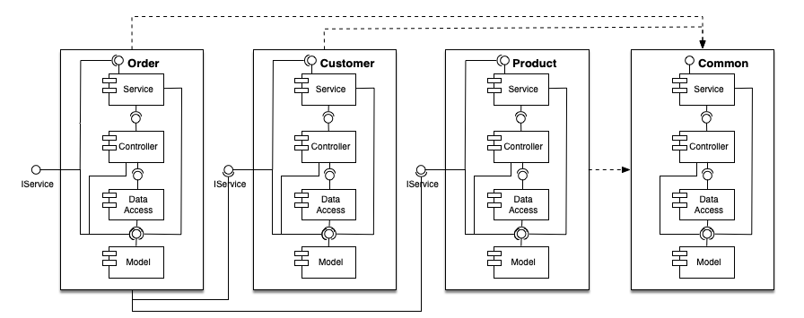
The different functional components are sitting within their own silos and dependencies between those are not cyclical, i.e. there is a clear hierarchy between the silos. You could also describe that as vertical layering; or as micro-services within a monolith.
Unfortunately many software system fail at verticalization The main reason is that there is nobody to force you to organize your code into silos. Since it is hard to do this in the right way the boundaries between the silos blur and functionality that should reside in a single silo is spread out over several of them. That in turn promotes the creation of cyclic dependencies between the silos. And from there maintainability goes down the drain at an ever increasing rate.
Defining a new metric
Now how could we measure verticalization? First of all we must create a layered dependency graph of the elements comprising your system. We call those elements “components” and the definition of a component depends on the language. For most languages a component is a single source file. In special cases like C or C++ a component is a combination of related source and header files. But we can only create a proper layered dependency graph if we do not have cyclic dependencies between components. So as a first step we will combine all cyclic groups into single nodes.
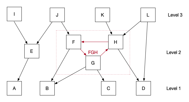
In the example above nodes F, G and H form a cycle group, so we combine them into a single logical node called FGH. After doing that we get three layers (levels). The bottom layer only has incoming dependencies, to top layer only has outgoing dependencies. From a maintainability point of view we want as many components as possible that have no incoming dependencies, because they can be changed without affecting other parts of the system. For the remaining components we want them to influence as few as possible components in the layers above them.
Node A in our example influences only E, I and J (directly and indirectly). B on the other hand influences everything in level 2 and level 3 except E and I. The cycle group FGH obviously has a negative impact on that. So we could say that A should contribute more to maintainability than B, because it has a lower probability to break something in the layers above. For each logical node  we could compute a contributing value
  to a new metric estimating maintainability:
![\[ c_i = \frac{size(i) * (1 - \frac{inf(i)}{numberOfComponentsInHigherLevels(i)})}{n} \]](https://blog.hello2morrow.com/wp-content/ql-cache/quicklatex.com-07ada843a06f6ae7e04f933563cbb45b_l3.png "Rendered by QuickLaTeX.com")
where  is the total number of components,
  is the number of components in the logical node (only greater than one for logical nodes created out of cycle groups) and
  is the number of components influenced by .
Now lets compute for node A:
![\[ c_A = \frac{1 * (1 - \frac{3}{8})}{12} \]](https://blog.hello2morrow.com/wp-content/ql-cache/quicklatex.com-1cea367957ea404c1e1ec0ff440a4245_l3.png "Rendered by QuickLaTeX.com")
If you add up for all logical nodes you get the first version of our new metric “Maintainability Level”  :
:
![\[ ML_1 = 100 * \sum_{i=1}^{k} c_i \]](https://blog.hello2morrow.com/wp-content/ql-cache/quicklatex.com-21147286fce569341ba4b23f96f3d331_l3.png "Rendered by QuickLaTeX.com")
where  is the total number of logical nodes, which is smaller than if there are cyclic component dependencies. We multiply with 100 to get a percentage value between 0 and 100.
Since every system will have dependencies it is impossible to reach 100% unless all the components in your system have no incoming dependencies. But all the nodes on the topmost level will contribute their maximum contribution value to the metric. And the contributions of nodes on lower levels will shrink the more nodes they influence on higher levels. Cycle groups increase the amount of nodes influenced on higher levels for all members and therefore have a tendency to influence the metric negatively.
Now we know that cyclic dependencies have a negative influence on maintainability, especially if the cycle group contains a larger number of nodes. In our first version of we would not see that negative influence if the node created by the cycle group is on the topmost layer. Therefore we add a penalty for cycle groups with more than 5 nodes:
![\[ penalty(i) = \begin{cases} \frac{5}{size(i)},& \text{if } size(i)>5\\ 1, & \text{otherwise} \end{cases} \]](https://blog.hello2morrow.com/wp-content/ql-cache/quicklatex.com-20fc41099c5de33d1bdf92cc05a0e296_l3.png "Rendered by QuickLaTeX.com")
In our case a penalty value of 1 means no penalty. Values less than 1 lower the contributing value of a logical node. For example, if you have a cycle group with 100 nodes it will only contribute 5% ( ) of its original contribution value. The second version of now also considers the penalty:
![\[ ML_2 = 100 * \sum_{i=1}^{k} c_i * penalty(i) \]](https://blog.hello2morrow.com/wp-content/ql-cache/quicklatex.com-789c4c430b2dbcf475e4bd54b55a1c7a_l3.png "Rendered by QuickLaTeX.com")
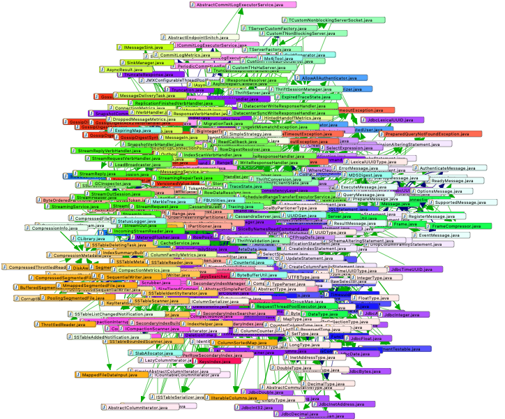
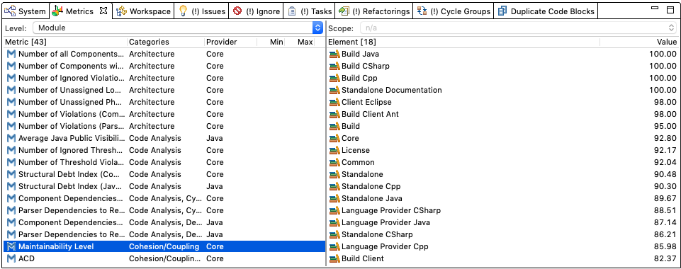
This metric already works quite well. When we run it on well designed systems we get values over 90. For systems with no recognizable architecture like Apache Cassandra we get a value in the twenties.
Fine tuning the metric
When we tested this metric we made two observations that required adjustments:
- It did not work very well for small modules with less than 100 components. Here we often got relatively low values because a small number of components increases relative coupling naturally without really negatively affecting maintainability.
- We had one client Java project that was considered by its developers to have bad maintainability, but the metric showed a value in the high nineties. On closer inspection we found out that the project did indeed have a good and almost cycle free component structure, but the package structure was a total mess. Almost all the packages in the most critical module were in a single cycle group. This usually happens when there is no clear strategy to assign classes to packages. That will confuse developers because it is hard to find classes if there is no clear package assignment strategy.
The first issue could be solved by adding a sliding minimum value for if the scope to be analyzed had less than 100 components.
![\[ ML_3 = \begin{cases} (100 - n) + \frac{n}{100} * ML_2,& \text{if } n<100\\ ML_2, & \text{otherwise} \end{cases} \]](https://blog.hello2morrow.com/wp-content/ql-cache/quicklatex.com-6f6fa9860b66184d12e7cd6088384cd9_l3.png "Rendered by QuickLaTeX.com")
where is again the number of components. The variant can be justified by arguing that small systems are easier to maintain in the first place. So with the sliding minimum value a system with 40 components can never have an value below 60.
The second issue is harder to solve. Here we decided to compute a second metric that would measure package cyclicity. The cyclicity of a package cycle group is the square of the number of packages in the group. A cycle group of 5 elements has a cyclicity of 25. The cyclicity of a whole system is just the sum of the cyclicity of all cycle groups in the system. The relative cyclicity of a system is defined as follows:
![\[ relativeCyclicity = 100 * \frac{\sqrt{sumOfCyclicity}}{n} \]](https://blog.hello2morrow.com/wp-content/ql-cache/quicklatex.com-cd0454b9703bf98959107c582d7a2fe2_l3.png "Rendered by QuickLaTeX.com")
where is again the total number of packages. As an example assume a system with 100 packages. If all these packages are in a single cycle group the relative cyclicity can be computed as  which equal 100, meaning 100% relative cyclicity. If on the other hand we have 50 cycle groups of 2 packages we get
  – approx. 14%. That is what we want, because bigger cycle groups are a lot worse than smaller ones. So we compute
  like this:
![\[ ML_{alt} = 100 * (1 - \frac{\sqrt{sumOfPackageCyclicity}}{n_p}) \]](https://blog.hello2morrow.com/wp-content/ql-cache/quicklatex.com-62668681f7b1bcf32de8de2a8a2d91a3_l3.png "Rendered by QuickLaTeX.com")
where  is the total number of packages. For smaller systems with less than 20 packages we again add a sliding minimum value analog to
  .
.
Now the final formula for ML is defined as the minimum between the two alternative computations:
![\[ ML_4 = min(ML_3, ML_{alt}) \]](https://blog.hello2morrow.com/wp-content/ql-cache/quicklatex.com-37d0ae55ca2ad6e80add2fbae053ae6b_l3.png "Rendered by QuickLaTeX.com")
Here we simply argue that for good maintainability both the component structure and the package/namespace structure must well designed. If one or both suffer from bad design or structural erosion, maintainability will decrease too.
Multi module systems
For systems with more than one module we compute ML for each module. Then we compute the weighted average (by number of components in the module) for all the larger modules for the system. To decide which modules are weighted we sort the modules by decreasing size and add each module to the weighted average until either 75% of all components have been added to the weighted average or the module contains at least 100 components.
The reasoning for this is that the action usually happens in the larger more complex modules. Small modules are not hard to maintain and have very little influence on the overall maintainability of a system.
Try it yourself
Now you might wonder what this metric would say about the software you are working on. You can use our free tool Sonargraph-Explorer to compute the metric for your system written in Java, C# or Python. is currently only considered for Java and C#. For systems written in C or C++ you would need our commercial tool Sonargraph-Architect.
Of course we are very interested in hearing your feedback. Does the metric align with your gut feeling about maintainability or not? Do you have suggestions or ideas to further improve the metric? Please leave your comments below in the comment section.
References
The work on ML was inspired by a paper about another promising metrics called DL (Decoupling Level). DL is based on the research work of Ran Mo, Yuangfang Cai, Rick Kazman, Lu Xiao and Qiong Feng from Drexel University and the University of Hawaii. Unfortunately a part of the algorithm computing DL is protected by a patent, so that we are not able to provide this metric in Sonargraph at this point. It would be interesting to compare those two metrics on a range of different projects.
This is great! Are you going to produce an analyzer for Go?
We need some paying customers for Go language support that would justify such an investment.
It’s obviously not a one-size-fits-all metric, but it still seems like an interesting and broadly-useful approach.
Perhaps the weighting could be extended and made still more useful by using traditional complexity metrics (branch-counting, line-counting, etc.)?
I think it is better to keep it focussed on structure and maybe create a second metric to measure overall complexity.
Can you give me an example of the metric with component cycles? I tried to compute the metric manually but I can not get the same result as sonargraph.
Thank you.
Can you give me your example?
Perhaps it’s not very constructive, but… why would they patent this work? It seems bizarre, considering this topic is largely unappreciated in the industry and the adoption is difficult enough already.
They sell a tool that computes it, I guess they don’t want anybody to copy it…
2.5 years later – I’m curious, what’s the lessons learnt from using this metric?
Some of our customers use it to monitor portfolios of projects and it is a good early warning indicator.
This article is so good I keep coming back to this article and rethinking it over and over again 🙂 I get the point about cycles, but don’t quite understand what are the strategies the manage the “degree of influence”.
In the article you say:
“From a maintainability point of view we want as many components as possible that have no incoming dependencies, because they can be changed without affecting other parts of the system. For the remaining components we want them to influence as few as possible components in the layers above them.”
I’m not sure that I understand how this can be achieved in a practical setting. The way I think about it – if component is influencing others it must be for a reason – what is the alternative? Would you have a practical example of how reducing influence can be achieved – for example two designs which achieve the same goal, but one has better ML than the other?
Thank you for your kind feedback. Regarding your question, a perfect score is not the goal, if you can keep it above 80% it is good enough. And to achieve a good score it is a good strategy to isolate large classes that implement functionality by interfaces. So those classes will not be called directly and therefor have no i coming dependencies. Interface changes are less likely than implementation changes. Another thing that helps is keeping vertical boundaries (Domain Driven Design), i.e. minimize dependencies between domains. You should consider this metric a coupling indicator and have a look at coupling issues when the value is in a downward trend.