Sonargraph-Enterprise is designed to allow stake-holders to track important software quality metrics over time. The idea is that this would enable the early detection of harmful trends so that issues can be fixed while they are still easy to fix. The metrics displayed by Sonargraph-Enterprise can be fully customized by the user. However, in this article I will explain the “default” profile that comes with a set of preselected metrics that cover important aspects of code health and quality.
When you navigate to Sonargraph-Enterprise in your browser, that first thing you will see is a list of all projects that have uploaded data to Sonargraph-Enterprise. To add a project to this list you need use Sonargraph-Build to upload a set of data typically once a day. The details are described in the Sonargraph-Build manual.
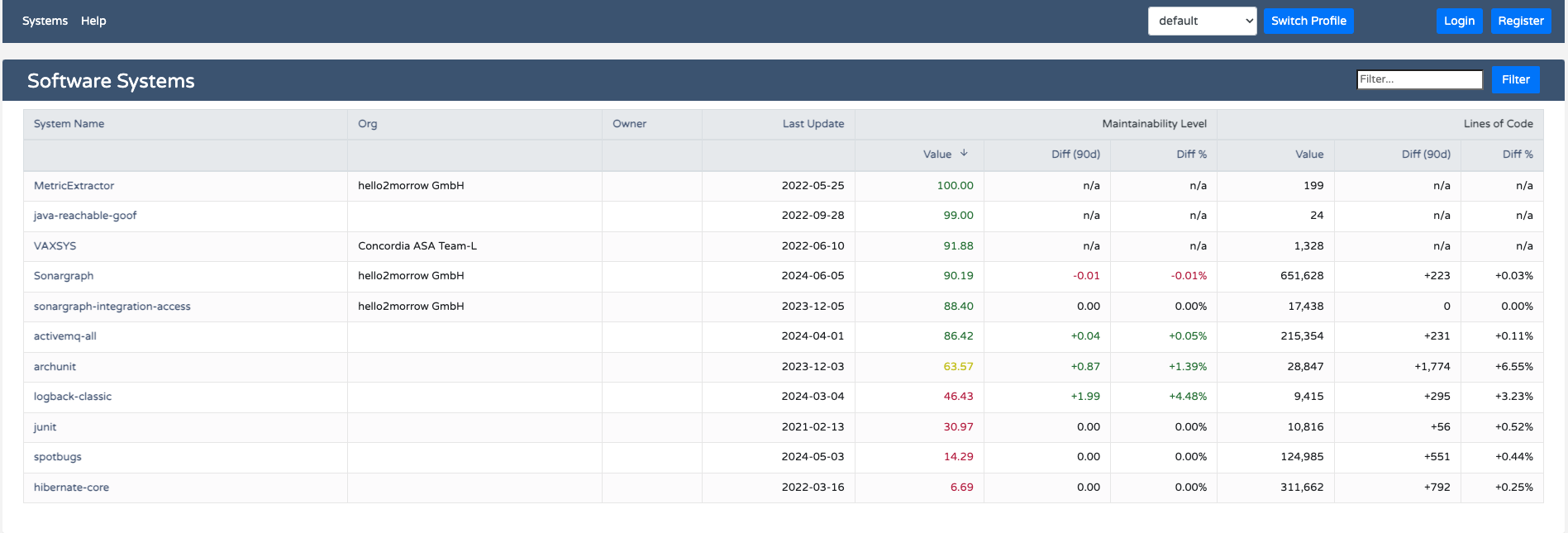
As you can see for each project we display the name, organizational unit and owner, the date of the last update and two metrics that are compared over a configurable number of days. The default would be 90 days, but can be changed by defining a new profile. By clicking on any column header you can sort the list by the values in that column. A second click will reverse the sort order.
In the default profile we decided to use “Maintainability Level” (ML) and “Lines of Code” (LoC). ML is a relatively new metric that we designed together with some of our customers to measure the overall maintainability of a software system by analyzing the dependency structure. We have published a blog article that describes how the metric is calculated in detail. In short it is a percentage value with 100% marking the best possible value. You should be concerned if it falls below 50% and aim to keep it above 70%. In the list above you can see that the project “hibernate-core” scores under 7%. If you get that low it will be very difficult to bring the value back up because you have reached the final stages of a big ball of mud. On the system level the metric is calculated as a weighted average of the ML values of all the modules in a system.
Sonargraph-Enterprise allows you to establish a metric-based feedback loop. You can follow trends and react if metrics turn yellow or red. The earlier you do that the less effort will be needed to address the problem.
The second metric “Lines of Code” is obvious. It tells you how big a system is and how much changes are happening.
Once you click on one of the systems you will get a more detailed view with 10 different metrics:
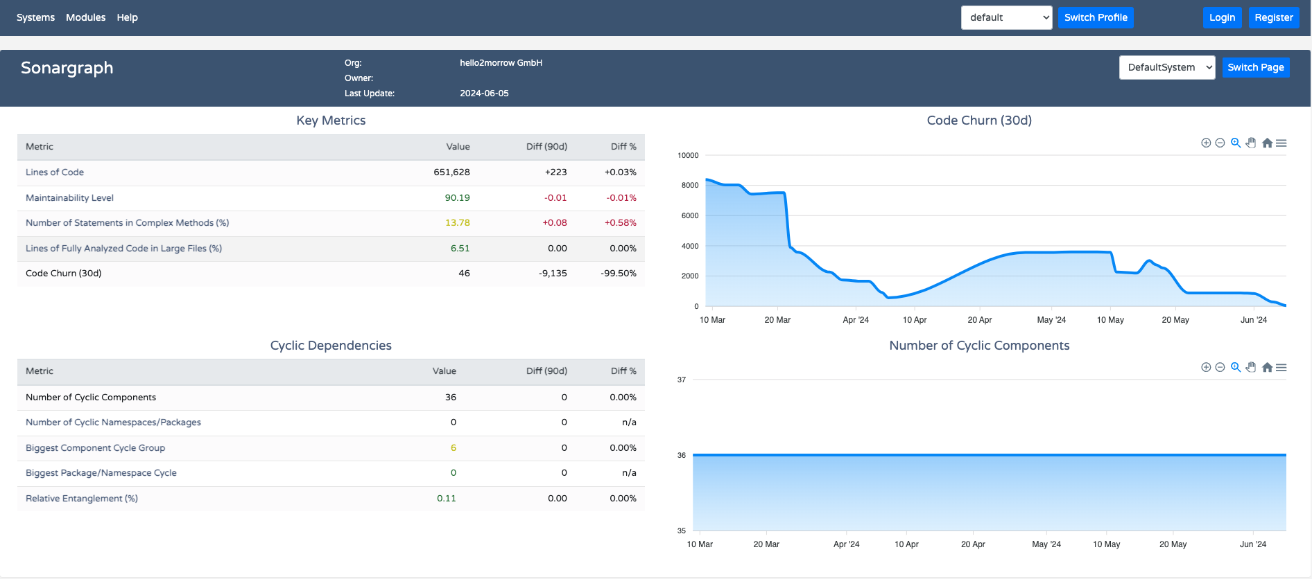
You see two blocks which we call metric sets. These sets are configurable, but in that case they are pre-configured s part of the default profile. On the right side you see how the currently selected metric in the set changed over time The default time window is 90 days, but also can be changed by creating a new profile.
Lets go through the first metric set called “Key Metrics”:
- Lines of Code: counts all code lines except for empty lines and comments.
- Maintainability Level: has already been explained above. The best way to improve the value is to reduce overall coupling. The best way to do that is to disentangle cyclic dependencies. We will cover that aspect further down. Since this metric is weighted average of the modules comprising the system, it is a good idea to break it down to the module level. To do that just click on “Modules” on the top of the screen and you will get a list of modules sorted by ML. Click on the column header to change the sort order so that the “worst” module will appear on the top of the list.
- Number of Statements in Complex Methods: here we measure what percentage of your code base is inside of “complex” methods or functions. We consider a method to be complex, if either the metric “Cyclomatic Complexity” is above 15 or the indentation depth is greater than 4. Of course we want this metric to be as small as possible. In our example system the value is over 13%, therefore marked in yellow. Overly complex code will make developers spend kore time trying to understand code and therefor leaves less time for changing or adding code. The default thresholds of 15 and 4 can be changed inside of Sonargraph-Architect.
- Lines of Fully Analyzed Code in Large Files: here we look at what percentage of your code base is located in large source files. By default a source file is considered to be large if it hs more than 1,000 lines of code, but again that threshold can be changed in Sonargraph-Architect. Large source files can be problematic because they tend to increase coupling considerably. Typically those large files contain God classes that have too much functionality. Sometimes those files are generated. In that case you can setup an issue filter in Sonargraph that will exclude those generated files from influencing the metric. The details are described in another blog article. Again we would like to keep this value as small as possible. In our example it is under 7% and therefore displayed in green.
- Code Churn (30d): this measures how many lines have been added, changed or removed from the project in the last 30 days. A value is only provided if you are using Git as your version control system. This number measures development activity over time. Projects under active development will have higher values than inactive project.
The second metric set is focussing on cyclic dependencies (as the name implies). A cyclic dependency is created when two source files mutually depend on each other. This would form the smallest possible cycle group of two elements. Of course those cycle groups can grow. The reason why “hibernate-core” has such a low value of ML is caused by a gigantic cycle group of more than 1,000 Java files.
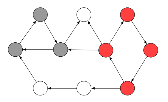
This graphic shows a dependency graph where the circles could be either single source files or packages or name spaces. We have two cycle groups there, one in red and one in gray.
Detecting and analyzing cyclic dependencies is a very reliable method to detect the level of structural or architectural erosion in a software system. In short, the bigger the cycle groups and the more elements are involved in those cycles, the bigger the problem is. Smaller cycle groups are less harmful then larger cycle groups. When looking at cycles between source files or classes it is preferable to have them all within the same package or name space. Large cycle groups are a good indicator for discovering software rot.
There are plenty of reason why cyclic dependencies, especially larger cycle groups are harmful for software maintainability:
- Modularity is decreased.
- It becomes impossible to test functionality in isolation.
- Developers need way more time to understand a tightly coupled code base.
- It becomes much harder to harden the code against vulnerabilities.
- If the project passes from one team to another the new team will have great difficulties maintaining that code in a good way.
- The dependency on the availability or the original developers becomes critical, because they are the only ones with na deeper understanding of the code base.
Structural/architectural erosion is caused by these cyclic dependencies and can be considered the most toxic form or technical debt. The reason is that fixing an eroded structure requires global refactorings of the code base, which is risky and takes a lot of effort. Other forms of technical debt are much more localized and can therefore be fixed by local changes.
Therefor this second metric set focusses on that particular aspect. We don’t even have to look at conformance to architectural models. But we can assume that if the values are good the team has a good handle on the overall architecture and structure of the system. And having an architectural model based on Sonargraph’s architecture DSL will automatically ensure that your system can never erode into a big ball of mud. I highly recommend to make the creation of such models mandatory for each development team.
Now lets look in the metrics in that set:
- Number of cyclic components: counts the number of components involved in cyclic dependencies. the definition of “component” depends on the language. For most languages a “component” is a single source files. For C/C++ a component if a combination of source and header files and typically contains one header and one source file.
- Number of cyclic namespaces/packages: here we count the number of namespaces or packages involved in cyclic dependencies with other namespaces or packages. Namespace and package cycles are worse then component cycles and should be avoided. They can be a side effect of component cycles if the components in a cycle belong to several packages or namespaces. They also can be caused by classes assigned to the wrong namespace or package. Often the lack of a clear strategy for defining namespaces or packages also plays an important role.
- Biggest component cycle group: here we count the number of components in the biggest cycle group of the system. Once they reach a certain size they are like code cancer and grow bigger and bigger until your whole code base turns into a big ball of mud. We consider cycle groups with more than 5 elements to be critical, i.e. they should be urgently disentangled.
- Biggest package cycle group: analog to the metric above except that we count the number or namespaces/packages in the biggest namespace/package cycle group. We recommend to totally avoid namespace or package cycles, so tis number should be zero.
- Relative Entanglement (%): here we take the average of two metrics (which I will explain below): “Relative Cyclicity Components” and “Relative Cyclicity for Packages/Namespaces”. You want to keep that value as small as possible. Larger values (over 20%) indicate that your system is deteriorating into a big ball of mud. (This metric was recently improved as described in this post)
Relative cyclicity is calculated by first adding up the cyclicity of all cycles groups in a given scope (system or module – in Sonargraph terms a system can contain many modules, at least one). The cyclicity of a cycle group is the square number of the number of elements in the group. For example the cyclicity of a cycle group with 4 elements is 16.
This leads us to the formula for relative cyclicity:
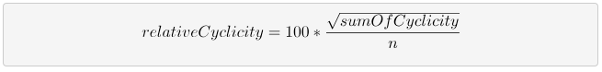
Lets try that formula with a hypothetical example. Lets assume we have a system with 50 source files, all of which are involved in one big cycle group of 50 elements. In that case “sumOfCyclicity” would be 2.500 (50 * 50). The square root gives a value of 50, which will then be divided through the total number of elements in that system, in our case 50. So relative cyclicity would be 100%, the worst possible value.
Now lets assume a similar system with 50 source files, but instead of one big cycle of 50 elements we have 25 cycles of 2 elements. In that case the “sumOfCyclicity” would be 100 (25 * 4). In that case the formula would evaluate to 20%.
Now we can see the usefulness of that metric. Even though all source files in both examples are involved in cyclic dependencies, the second value is much better caused by the fact that you could cut the second system into 25 individual parts, while the first system cannot be sub-divided since everything is in one big cycle.
Thank you for reading this article to the end. If you have questions or comments you can add them below.