Almost everyone who worked in software development for a while has come in contact with the dreaded big ball of mud (BBoM). If you are not familiar with the term, it describes software systems that have lost their architectural cohesion and suffer from extreme coupling and large cyclic dependency groups. That makes it much harder to do any changes on those systems, because everything is literally connected to everything else. Therefor it requires developers spending almost all their time trying to understand code before they can risk doing changes. And even then, the chance of regression bugs stay pretty high. If a system reaches this state, doing changes becomes so expensive, that rewriting the system from scratch might be cheaper than maintaining the old system. Unfortunately, very often it is not possible to rewrite the system, because the users can’t wait for years for a system replacement. This puts many development organization in a very uncomfortable place.
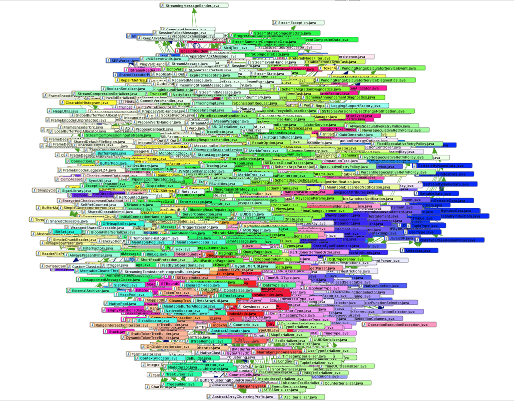
A big ball of mud visualized by Sonargraph
The screenshot above shows a pretty big big ball of mud, where several hundred Java files form a gigantic cycle group. As you can imagine, it will probably be very difficult o untangle this dependency jungle. A much better way to tackle this problem is to use metric based feedback loops to monitor a set of key metrics during active development that would tell us early if we are headed in the direction of the BBoM. This article will introduce one metric, that was designed for this purpose.
But before we introduce this metric let me first explain another metric that is used as an input for the new metric. This metric is called “Relative Cyclicity”. Relative cyclicity is calculated by first adding up the cyclicity of all cycles groups in a given scope (system or module – in Sonargraph terms a system can contain many modules, at least one). The cyclicity of a cycle group is the square number of the number of elements in the group. For example the cyclicity of a cycle group with 4 elements is 16. This leads us to the formula for relative cyclicity:

Lets try that formula with a hypothetical example. Lets assume we have a system with 50 source files, all of which are involved in one big cycle group of 50 elements. In that case “sumOfCyclicity” would be 2.500 (50 * 50). The square root gives a value of 50, which will then be divided through the total number of elements in that system, in our case 50. So relative cyclicity would be 100%, the worst possible value.
Now lets assume a similar system with 50 source files, but instead of one big cycle of 50 elements we have 25 cycles of 2 elements. In that case the “sumOfCyclicity” would be 100 (25 * 4). In that case the formula would evaluate to 20%.
Now we can see the usefulness of that metric. Even though all source files in both examples are involved in cyclic dependencies, the second value is much better caused by the fact that you could cut the second system into 25 individual parts, while the first system cannot be sub-divided since everything is in one big cycle. To come back to the big ball of mud analogy, 100% relative cyclicity is the worst possible BBoM.
Ever increasing cyclic dependencies are an excellent indicator, that a system is deteriorating towards a BBoM. Therefore measuring relative cyclicity can be used to quantify where we are on the spectrum between a BBoM and a well designed system, that is easy to maintain. But we have yo be aware, that there are different categories of circular dependencies:
- Cycles between source files.
- Cycles between programming elements like classes or functions.
- Cycles between namespaces or packages.
- Cycles between source directories.
For example, we could have clean dependencies on the source file level, while having lots of cycles between namespaces or packages. So it would not be enough to just look at one category of circular dependencies, we have to look at all of them and calculate a combined value out of them.
There is also an interesting difference between the first two categories and the last two categories. The first two create what we call “real cycles”. If a class A is using a class B, B is using C and C uses A we have a real cycle of 3 elements. Often enough package or namespace cycles are not real cycles. That means the cycle can be solved by just moving elements between namespaces or packages.

For example, if you look at the two namespaces “Alpha” and “Beta” above you can see, that although they depend on each other, the circular dependency is not caused by a real cycle. That would only be the case if there was also a dependency from B to A. So here the cycle can be broken by just moving B to “Beta” or C to “Alpha”. There is no need to cut any dependencies between A, B or C.
We consider “real” cycles to be a bigger problem. To untangle them you always need to cut some dependencies between the elements forming the cycle. So while package, namespace or directory cycles can be caused by real cycles, often enough moving elements around is enough to break the cycle.
Now lets introduce our BBoM detecting metric, which we will name “Relative Entanglement”. It ranges between 0 and 100%. The calculation is based on two inputs. One input covers real cycles and therefore uses the arithmetic average of relative cyclicity of the first two cycle categories (source files and programming elements). The second input uses the other two categories. For some languages, like Java, it does not make sense to calculate directory cycles, because the relation between directories and packages is hard coded by the language. For other languages, like C# or C++, both categories make sense.
So again, we take the arithmetic average of relative cyclicity for the last two cycle categories (in Java we only use relative cyclicity of packages) to come up with our second input value. Then we create a weighted average of our two inputs, where real cycles have a weight of 60% and all other cycles are weighted at 40%.
After testing the metric on many different systems we came to the conclusion, that it is an excellent indicator to indicate how much a system has eroded towards the BBoM. Values under 10% are ok, although I’d never allow my systems to go over 5%. Value between 10% and 20% are early stages of the BBoM. The system is still manageable and maintainable, but it already contains a few cycle groups with dozens of elements. Anything above 50% can be considered to be really problematic.
So if you want to avoid your system ending up as the dreaded BBoM, you could just track this metric in your nightly build and break the build as soon as the value grows over your comfort level. The metric can be measured using Sonargraph (version 15.2.0 or higher) and is also available in our free version Sonargraph-Explorer. It is also prominently displayed in the top right box of the Sonargraph dashboard.

The Sonargraph dashboard displays relative entanglement in the “Structure” box.
We just recently updated our dashboard and the changes are described in this article. Now if you are curious where your system stands with respect to this metric I recommend creating an account on www.hello2morrow.com and either get a free two-weeks evaluation license of Sonargraph-Architect or a free license of Sonargraph-Explorer. The free version supports Java/Kotlin, C#, TypeScript and Python. The commercial version also supports C and C++.
Chances are that you will find some level of cyclic dependencies in your system using Sonargraph. If you use Sonargraph-Architect you can use its capability to do virtual refactorings to untangle the cycles step by step. The earlier you do that the easier it will be. We even created a tutorial video so that you can see how this is done.
If you have question or want to give us your feedback about this article, please leave a comment below.